Making Choropleth Maps in Stata

A Choropleth map uses different colours or shading for different areas of a map to indicate average values for each area. For example – a map of Australia with each state as a separate area, each area coloured to represent the proportion of the population of Australia who live there. This example is shown below.

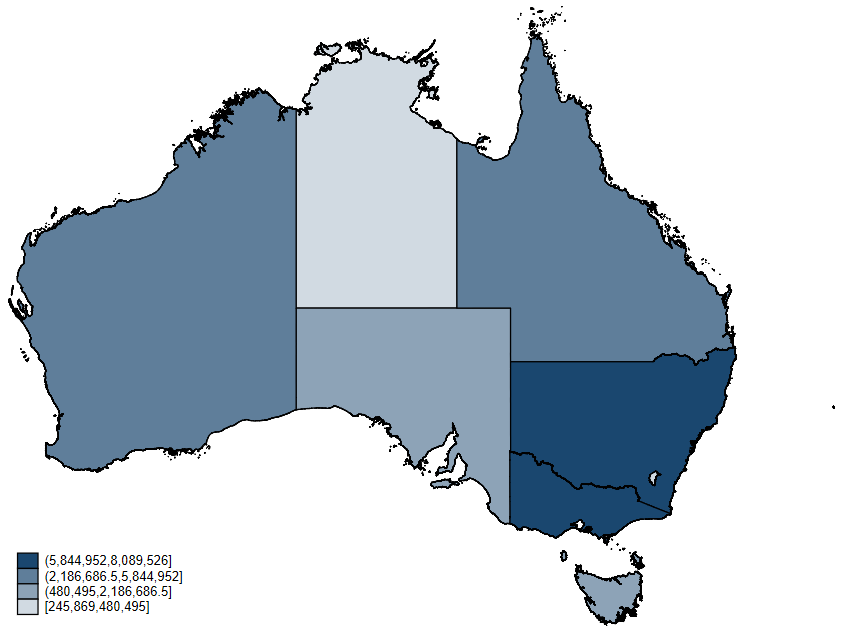
These maps are easy to make in Stata provided you have the GIS mapping shapefiles for the country or region you want to map. And of course you will need the data you want to make your choropleth map with. In the case of the map of Australia above, the population data is easily obtainable through Wikipedia, and the map files can be accessed through the Australian Bureau of Statistics.

Once you have your GIS shapefiles and your choropleth data, you can easily import the map files with the command spshape2dta and either frame-link or merge the choropleth data to create one spatial dataset. With this dataset set up, you use the grmap command to generate your map. Below I will go through the steps required to make the population map above.

Step 1: Find the GIS mapping shapefiles

For Australia, GIS shapefiles can be obtained through the ABS website
There are many different types of boundaries saved here, however we are only interested in the state and territory boundaries for our map. To get these, look for the “States and Territories - 2021 - Shapefile” and click the “Download ZIP” button on the right. A Zip file called “STE_2021_AUST_SHP_GDA2020” should download.
Open the zip file. Most Windows and Mac computers can open zip files easily, however if you are having trouble there are some free programs that will open zip files for you.
There are a whole bunch of files in the zip, however we are only interested in the database file (.dbf) and shapefile (.shp). Save these files in a location you know. I have saved mine in a folder called AUS, located in a folder called Maps in my Documents folder.

Step 2: Import the GIS mapping shapefiles using spshape2dta

The ESRI shapefile and database file I downloaded are called STE_2021_AUST_SHP_GDA2020.dbf and STE_2021_AUST_SHP_GDA2020.shp and they are saved in folder AUS located in a folder called Maps in my Documents folder. In order for this to work the database file and shapefile should have exactly the same name, just with different file extensions (one .dbf and one .shp). All ESRI files you download should be formatted like this, but if they are not make sure to rename them correctly. To import and convert these to Stata datasets I use the following command:

clear all
spshape2dta "C:\Users\Laura\Documents\Maps\AUS\STE_2021_AUST_GDA2020"

This gives the following output in the command pane:

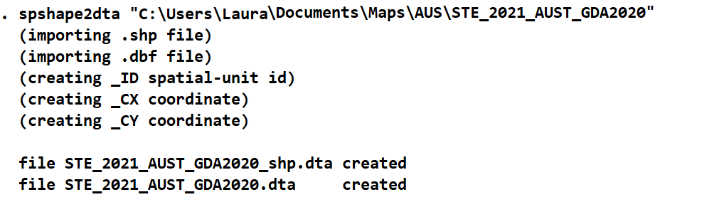
You will see from this that two Stata datasets are created. Make sure these always stay in the same folder together (if you move one you need to move both). The file you want to use is the regular file, in this case “STE_2021_AUST_GDA2020.dta”. DO NOT touch the file with “_shp.dta” on the end. This is what creates the map, any alterations will mean the map cannot be drawn.

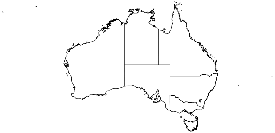
Now that the datasets have been converted in Stata, I am going to load the region dataset and draw a blank map of Australia to make sure my spatial data has imported correctly. In the command pane:

use "C:\Users\Laura\Documents\Maps\AUS\STE_2021_AUST_GDA2020.dta", clear
grmap, activate
grmap

Step 3: Merging or frame-linking choropleth data

There are many ways to get the population data from Wikipedia. You can input the data manually; write a Java/C/C++ Stata plugin to scrape the data; use Python in Stata interactively to scrape the data; import using Microsoft Excel; or use an online tool.

For this example I use the online tool wikitable. I input the wikipedia webpage, click convert, and download tables 2 and 3 as a csv. To then get this into Stata I use the following commands:

clear all
import delimited "C:\Users\Laura\Downloads\table-2.csv"
drop flag iso2 area governor premier v10
rename (statename abbrev population) (state state_code population)
save "C:\Users\Laura\Documents\Maps\AUS\aus_population_2019.dta", replace
import delimited "C:\Users\Laura\Downloads\table-3.csv", clear
drop flag iso2 postal area administrator chiefminister v11
rename (territoryname abbrev population) (state state_code population)
append using "C:\Users\Laura\Documents\Maps\AUS\aus_population_2019.dta"
replace population=subinstr(population, "," ,"",.)
destring population, replace
format population %16.0gc
save "C:\Users\Laura\Documents\Maps\AUS\aus_population_2019.dta", replace

Now I need to merge the data together. There are two ways of doing this, either with merge or by using the new frame link commands. For this example I am just going to merge the two files:

clear all
use "C:\Users\Laura\Documents\Maps\AUS\STE_2021_AUST_GDA2020.dta"
rename STE_NAME21 state
merge 1:1 state using "C:\Users\Laura\Documents\Maps\AUS\aus_population_2019.dta"
drop if _merge != 3
drop _merge
save "C:\Users\Laura\Documents\Maps\AUS\spatial_population_aus.dta", replace

Step 4: Generating a choropleth map

Now that I have my dataset together and set (either through merging or frame-linking), it is as simple as giving the command grmap along with the variable name that I would like to map. It is worth noting here that if this is the first time you have ever used grmap on your current Stata you will need to activate it first with command grmap, activate. I did this for my version earlier in Step 2. Now let’s generate our population map! In the command pane:

grmap population

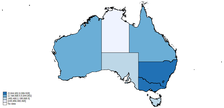
Now this map looks pretty good. However, if you are familiar with the population sizes for states and territories in Australia you may have noticed a problem with this map. The Australian Capital Territory (ACT), the small territory located entirely within New South Wales (NSW), has a population close to that of Tasmania (TAS). The ACT should be coloured a light blue, the same as TAS (the island below the rest of the country). But in this map it’s colour is the same as NSW.

Because of the way our map is generated, it has coloured NSW over the top of the ACT. This issue can be fixed, however it requires the creation of a second map using only the GIS map data for the ACT. Fortunately this is relatively easy to do. You will also need to specify your own colours in order for this to work. I am going to use various intensities of the colour navy for this map. In the command pane I type:

clear all
use "C:\Users\Laura\Documents\Maps\AUS\STE_2021_AUST_GDA2020.dta"
*Make a note of the _ID number that corresponds to the ACT
clear
use "C:\Users\Laura\Documents\Maps\AUS\STE_2021_AUST_GDA2020_shp.dta"
keep if _ID == 8
save "C:\Users\Laura\Documents\Maps\AUS\actmap.dta"
clear
use "C:\Users\Laura\Documents\Maps\AUS\spatial_population_aus.dta"
grmap population, fcolor(navy*0.2 navy*0.5 navy*0.7 navy*1.0) polygon(data("C:\Users\Laura\Documents\Maps\AUS\actmap.dta") fcolor(navy*0.2))

Now our map is complete and is correctly coloured. Usually you will not have a territory completely inside another region, so for most maps you draw with this feature it will work without any of the extra steps.