New and Improved Tables in Stata - An Introduction
Stata recently introduced the collect command, which allows you to consume results generated by Stata commands and mould them into customised tables. Any command that returns results in r() or e() macros can be consumed by collect. A couple of examples are regression models (e.g. linear, logistic, generalized, etc.), summary statistics (using the improved table command), statistical tests (e.g. t-test, chi2, etc.), and much more.
To determine if a command has consumable results, first run your command followed by these commands:
return list
ereturn list
If either of these commands prints output to the results pane, then the initial command you ran has results that can be consumed by collect.
Any command output that is consumed by collect is saved into a collection. By default, the collect command will save your consumed results to a collection called “default”. We will cover collections in more detail in a different post. Once you have consumed results with the collect command, you can then use the collect layout command to set up the overall table structure (rows and columns). When Stata consumes a command output, it automatically assigns both dimension(s) and level(s) to each item. This is what you use to define your table structure.
A dimension is like an overarching group. For example if you run a linear regression, the “coefficient” and the “standard error” are both assigned to the “results” dimension. The variables and the constant from the regression are assigned to the “colname” dimension.
A level is an individual item within the dimension. So for a linear regression, the coefficient (referred to as _r_b) is a level within the “results” dimension. The standard error (referred to as _r_se) is another level within the “results” dimension. The different variable names and the constant (referred to as _cons) are all separate levels within the “colname” dimension.
By separating everything into dimensions and levels Stata allows you to assign different levels or dimensions to different columns, rows, or even multiple tables. This means that your output can be manipulated to appear in every possible combination.
How to Use:
You can either collect results into a collection using the collect: prefix, or you can run the collect command after you have already run a command.
To use the prefix:
collect: regress var1 var2
OR, run a command, then:
collect get r() e()
To set the layout of your table so you can preview what it looks like:
collect layout (row_dimension[level(s)]) (column_dimension[level(s)]) (table_dimension[level(s)])
NOTE: You are not required to specify [level(s)], if you only specify the dimension then only the default set of levels will be shown. The default set of levels doesn’t include everything that was collected and is specific to the command you have collected from.
For the following examples I use the collect command after I have run an estimation command, rather than using the collect: prefix. To start you may prefer to use the collect: prefix as it will automatically choose a default layout for your table and will give you an idea of what everything will look like. I am not using it here as I want to demonstrate the use of layout commands and the Tables Builder to shape your table.
Worked Example 1: A Default Linear Regression
In this example I am going to demonstrate the use of both the collect commands and the Stata menus/Tables Builder to create a simple table using linear regression output. I will use the Stata example dataset auto.dta.
To start I will collect output from a linear regression and structure a simple table.
Tables via Commands:
sysuse auto, clear
regress price mpg
return list
ereturn list
collect get r() e()
collect layout (result) (colname)
The layout command produces the following table output:

Tables via Menus:
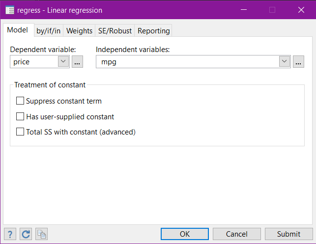
After loading the auto dataset with the sysuse auto command, we can run the regression through the Stata menus before collecting the output.
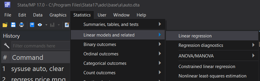
Statistics > Linear models and related > Linear regression
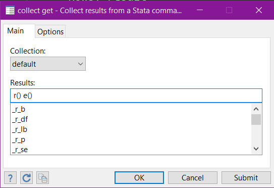
Now that we’ve run the regression, we can collect the output:
Statistics > Summaries, tables, and tests > Tables and collections > Collect results

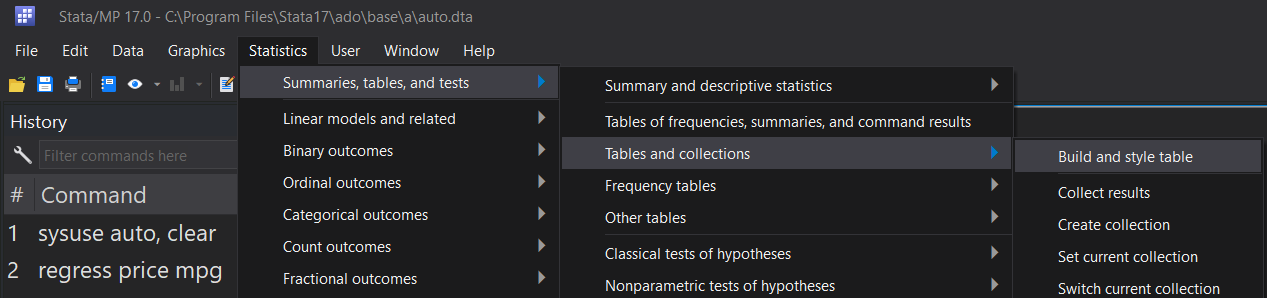
Once we’ve collected the output, we can open the Tables Builder to build our table layout:
Statistics > Summaries, tables, and tests > Tables and collections > Build and style a table
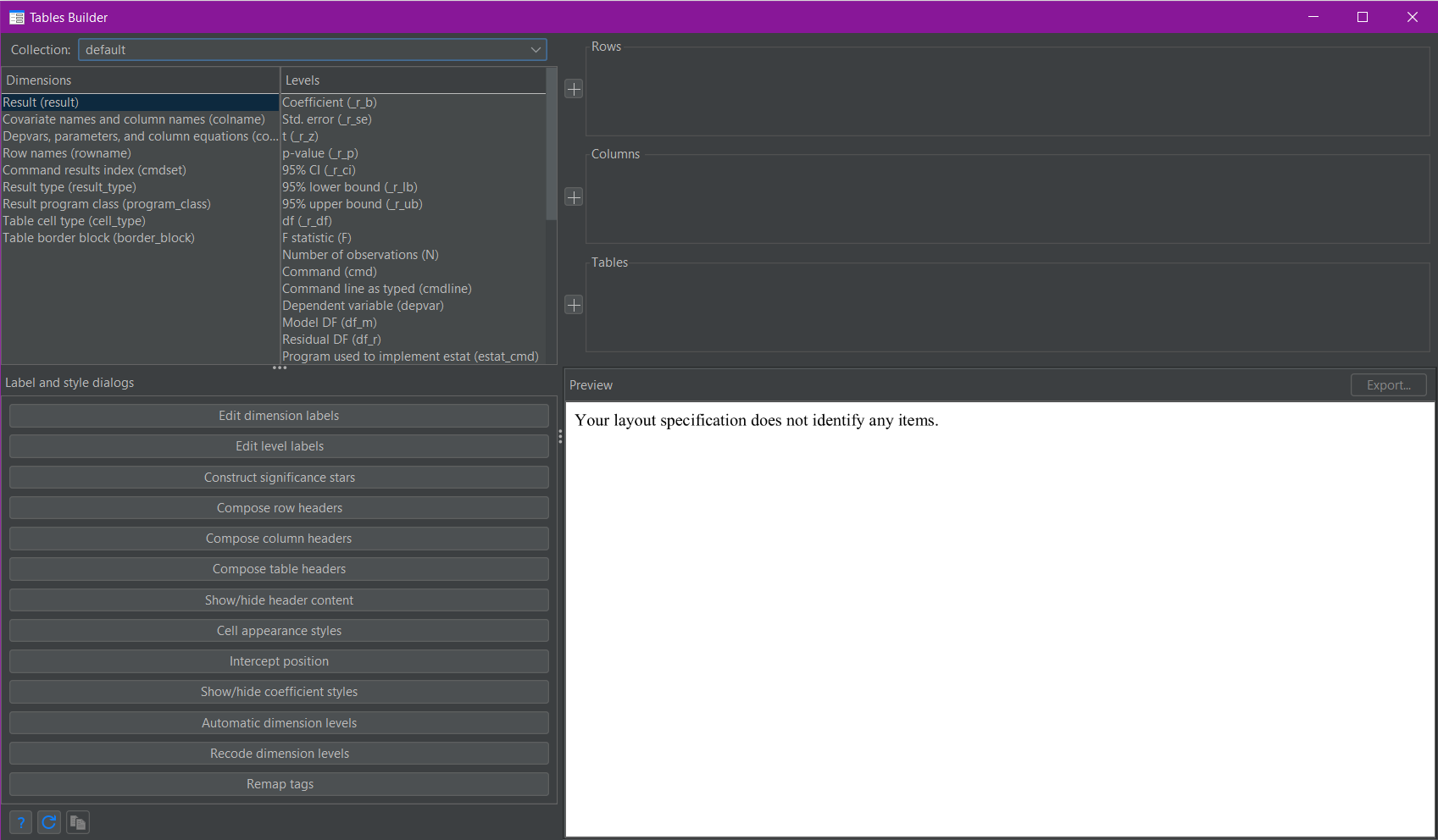
The dimensions and levels can be seen and selected in the top-left corner of the Tables Builder (shown above). In the top right are three squares, labelled rows, columns, and tables. This is where the selections of dimensions and levels are placed. The “plus” buttons to the left of the three squares are used to assign dimensions and/or levels to their chosen positions. In this case, I am only interested in the “result” and “colname” dimensions (the top two in the list). I click on the “result” dimension and click the plus next to rows, then I click on the “colname” dimension and click the plus next to columns.
This changes the view in the Tables Builder to the following:
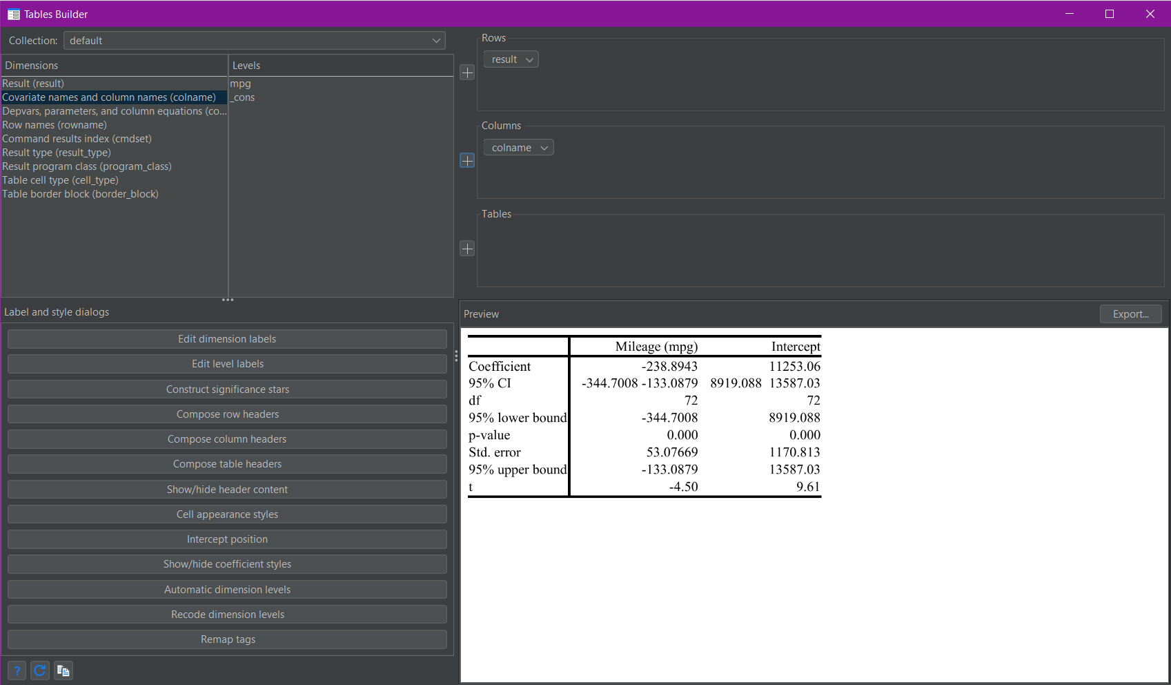
As you can see a preview of the resulting table is shown in the bottom-right of the Tables Builder (shown above).
There are a few things to note here. For the collect get command, it doesn’t matter what you specify beyond either r() or e(). You can specify a specific r() or e() result (or select one via the menu item) - for example r(table) to collect the matrix table - but this will still cause Stata to collect all the returned results in r() and/or e(). This is why I prefer to specify only r() and/or e() by themselves as this requires less typing. As I didn’t specify any levels for either of my dimensions in the layout, the default set for each dimension was shown. In this case, only the results from the third regression table output are shown, even though the information in the other two tables was also collected.
Worked Example 2: Selecting Levels
You can see the list of levels for each dimension in the Tables Builder. In addition to that, the following list of levels will be collected in the dimension result where appropriate:
- _r_b – coefficients or transformed coefficients reported by command
- _r_se – standard errors of _r_b
- _r_z – test statistics for _r_b
- _r_df – degrees of freedom for _r_b
- _r_p – p-values for _r_b
- _r_lb – lower bounds of confidence intervals for _r_b
- _r_ub – upper bounds of confidence intervals for _r_b
- _r_ci – confidence intervals for _r_b
- _r_cri – credible interval (CrI) of Bayesian estimates
- _r_crlb – lower bound of CrI of Bayesian estimates
- _r_crub – upper bound of CrI of Bayesian estimates
You can refer to this list in Stata by looking at the collect get help file.
I want to refine my previous table to show only the coefficient and p-value of the independent variable mpg. To do this I just need to add levels to the result and colname dimensions.
Tables via Commands:
The only command that changes from our previous example (1) is the last one, which we change to the following:
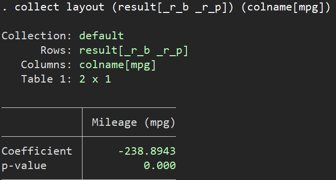
collect layout (result[_r_b _r_p]) (colname[mpg])
The layout command produces the following table output:
Tables via Menu:
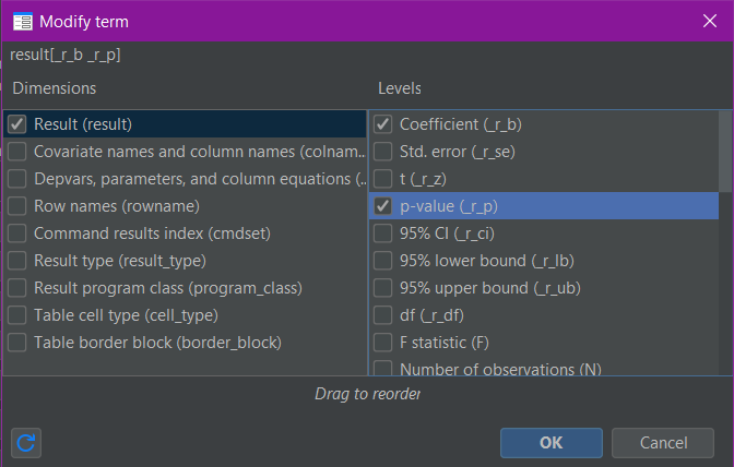
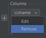
All the steps are the same as in the previous example (1), we just need to add our selected levels. The easiest way to do this is within the three squares (rows, columns, and tables) at the top left of the Tables Builder. The dimensions that we previously selected and moved into these squares have little drop-down arrows to the right of the dimension names. Click the drop-down arrow for the “result” dimension in rows and select “Edit”:

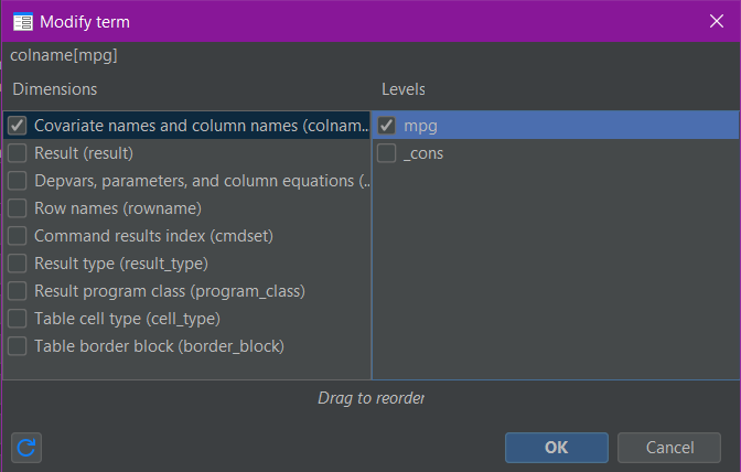
A box will appear and on the right of that box you can “tick” individual levels to select them:
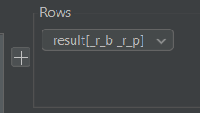
Once you click “OK”, the selections will show in the appropriate square of the Tables Builder:
We can also make the same selections for the “colname” dimension:

The Tables Builder then appears as follows with the appropriate table preview:
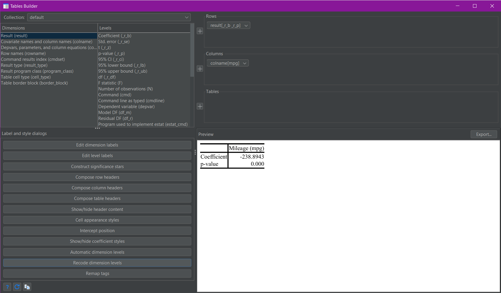
Dimensions and levels are the core to building complex tables in Stata 17 and newer. For the layout of tables I prefer to use the Tables Builder rather than just the commands. This allows for easier visualisation and manipulation to achieve the table structure I want. Once I have achieved my desired layout I can then use the corresponding layout command to reapply the layout where appropriate.