Melbourne Cup Performance Plots
This TechTip demonstrates how to create two complementary graphs in Stata to compare horse performance statistics for the 2026 Melbourne Cup.
The first graph is a heat map that visualises the comparison between multiple ratings for all 24 horses, and the second is a bar graph that combines these measures into a performance score and compares it with TAB betting odds to discover how you can get the best value out of your bet.
Preparing the Dataset
We begin with a dataset containing 15 variables for each horse:
. clear all

. use "horse.dta"

. describe

Contains data from horse.dta
 Observations:            24
    Variables:            15                  3 Nov 2026 11:48
-----------------------------------------------------------------------------------------------------------------------
Variable      Storage   Display    Value
    name         type    format    label      Variable label
-----------------------------------------------------------------------------------------------------------------------
horse           str40   %40s
country         str3    %9s
weight          float   %9.0g
trainer         str40   %40s
jockey          str40   %40s
tab_win         float   %9.0g
tab_place       float   %9.0g
age             int     %8.0g
gender          byte    %8.0g
barrier         int     %8.0g
starts          int     %8.0g
wins            int     %8.0g
seconds         int     %8.0g
thirds          int     %8.0g
rating          int     %8.0g
-----------------------------------------------------------------------------------------------------------------------
Sorted by:
As you can see, the variables country and trainer are currently stored as strings. Since there are some shared observations between individual horses, we can convert these into labelled numeric variables using encode.
. encode country, generate (country_code)

. encode trainer, generate (trainer_code)
This assigns a numerical code to each unique country or trainer whilst preserving its text as a value label. We can then replace the original string variables wih their encoded versions by reorganising their positions in the dataset:
. drop country

. drop trainer

.
. order country_code, after(horse)

. order trainer_code, before (jockey)

.
. rename country_code country

. rename trainer_code trainer
Next, the gender variable already contains numerical codes where gelding = 1, mare = 2 and stallion = 3. To ease data interpretation, we will use the label command to assign the respective genders to each number:
. label define gender_label 1 "gelding" 2 "mare" 3 "stallion"

. label values gender gender_label
Additionally, other useful measures of performance not included in the data are the percentage of race wins and the percentage of race places:
. generate win_percent = (wins/starts)*100

. generate place_percent = ((wins + seconds + thirds)/starts)*100
Creating the Horse Performance Heat Map
This heat map will compare the horses in the Melbourne Cup using four performance measures: rating, win percentage, place percentage and total races. It will use colour density to display how the values of individual obervations compare across all 24 horses.
Before generating the heat map, we need to use the preserve command to retain the original dataset whilst making temporary changes. Then, we need to convert each horse name into a labelled numeric value:
. preserve

. encode horse, generate(horse_id)
Because the four performance measures are all recorded on different scales, they need to be standardised before plotting them together. We use egen with the std() function to do this:
. egen z1 = std(rating)

. egen z2 = std(win_percent)

. egen z3 = std(place_percent)

. egen z4 = std(starts)
Now, each new variable represents the original measure expressed in standard deviations from its mean to allow colour intensity to represent relative differences between horses.
Since the four standardised variables are currently stored in seperate columns, we need to restructure them into long format in order to create the heat map:
. reshape long z, i(horse_id) j(metric)
(j = 1 2 3 4)

Data                               Wide   ->   Long
-----------------------------------------------------------------------------
Number of observations               24   ->   96
Number of variables                  22   ->   20
j variable (4 values)                     ->   metric
xij variables:
                           z1 z2 ... z4   ->   z
-----------------------------------------------------------------------------
The reshape long command combines z1, z2, z3 and z4 into one variable z. Finally, Stata’s twoway heatmap command can be used to display the standardised performance values:
. twoway heatmap z horse_id metric, ///
>     levels(11) crule(intensity) ecolor(navy) ///
>     xlabel(1 "Rating" 2 "Win %" 3 "Place %" 4 "Starts") ///
>     ylabel(1(1)24, valuelabel angle(0) labsize(small)) ///
>     yscale(reverse) ///
>     xtitle("") ytitle("") ///
>     title("Melbourne Cup Horse Performance") ///
>     graphregion(margin(l+15)) ///
>     xsize(11) ysize(9) ///
>         name(heatmap)

.
. restore
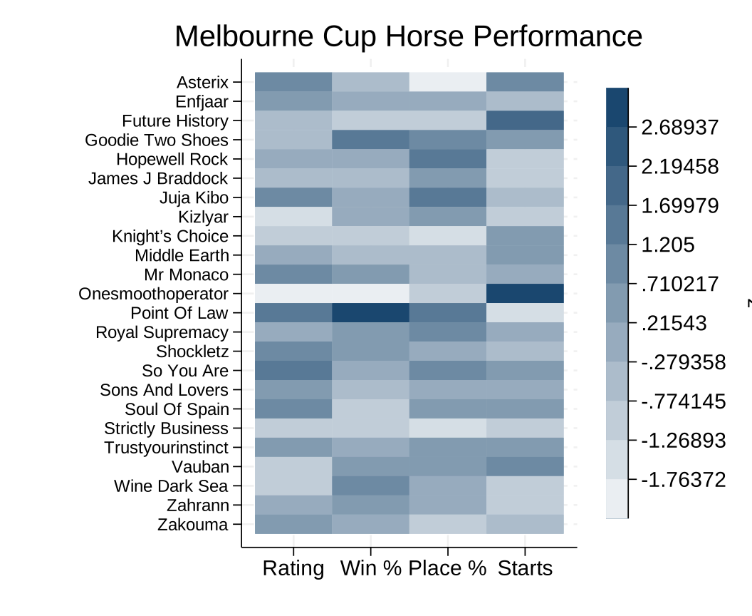
The finished heat map allows us to compare the relative performance measures of all 24 horses simultaneously, with darker colours indicating stronger historical records.
Creating the Betting Value Bar Graph
Now that we’ve visualised each horse’s historical performance, we can now compare these statistics with TAB win odds to identify potential valuabe bets. To do this, we calculate a composite performance score and compare the resulting ranking against the betting market ranking.
First, we calculate the combined number of races, wins and places across all 24 horses:
. egen total_starts = total(starts)

. egen total_wins = total(wins)

. egen total_places = total(wins + seconds + thirds)
Then, since horses with a small amount of career races could lead to a higher win percentage, we reduce that influence by adjusting each horses win and place place percentages towards the overall field averages. We start by definining the strength of this adjustment by introducing a local value, then calculate the adjusted percentages:
. local prior_starts = 10

.
. generate adj_win_pct = 100 * (wins + `prior_starts' * total_wins / total_starts) / (starts + `prior_starts')

. generate adj_place_pct = 100 * (wins + seconds + thirds + `prior_starts' * total_places / total_starts) / (starts + `
> prior_starts')
These calculations reduce extreme percentages for horses with fewer races while allowing horses with longer careers to retain more of their results. Next, we need to standardise the horses ratings with the two adjusted percentages then combine them into one composite score:
. egen z_rating = std(rating)

. egen z_win = std(adj_win_pct)

. egen z_place = std(adj_place_pct)

.
. generate form_score = 0.50*z_rating + 0.25*z_win + 0.25*z_place
This score assigns 50% weighing to horse rating and 25% rating to both adjusted win and place percentages. A higher form_score represents a stronger combined performance.
Then, to compare historical performance with with TAB’s betting market expectations, we create individual rankings for both a horses performance score and TAB win odds (with smaller odds reciving higher rankings). From this, the difference between the two rankings is calculated:
. egen form_rank = rank(-form_score)

. egen market_rank = rank(tab_win)

.
. generate value_gap = market_rank - form_rank
A positive value_gap indicates the horse rank more favourably according to its peformance score than according to its position in the betting market. Therefore, the horse with the largest value_gap will outperform its betting odds, providing the best value from placing a bet.
These ranking differences can be displayed using Stata’s graph hbar command:
. graph hbar (asis) value_gap, ///
>     over(horse, sort(1) descending ///
>     label(labsize(vsmall))) ///
>     title("Melbourne Cup: Potential Value Candidates") ///
>     subtitle("Career performance versus TAB win odds") ///
>     ytitle("Market rank minus form rank") ///
>     bar(1, color(navy)) ///
>     xsize(11) ysize(9) ///
>         name(value)
The (asis) option plots each horses calculated value_gap directly, rather than calculating a summary statistic. Then, the over() option displays one bar per horse and sorts the horses according to their ranking differences. The resulting graph will look like this:
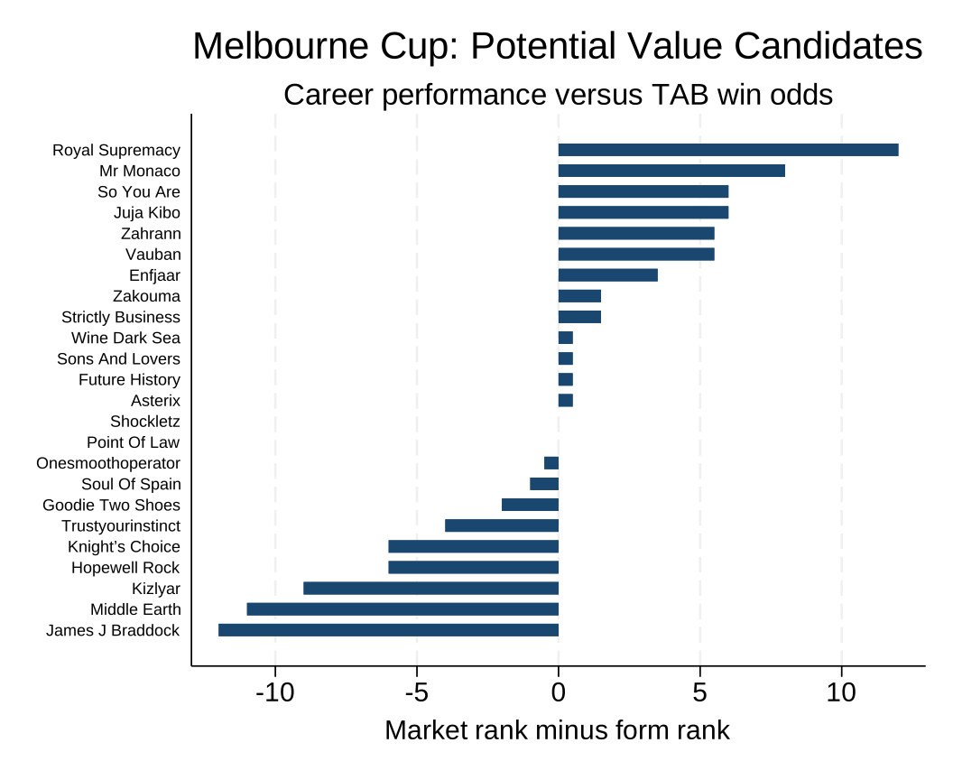
As you can see, Royal Supremecy ranks 8th according to its performance score but 20th according to TAB’s betting market, producing a value_gap of +12 and making it the most profitable horse.
Summary
Together, the two graphs provide different perspectives on the Melbourne Cup feild. The heat map allows us to compare multiple performance statistics similtaneously, whilst the horizontal bar graph combines weighted statistics into a ranking and compares that to TAB win odds.
However, the value graph does not incorportate factors such as barrier position, weight, age, trainer or country, so more calculations must be done to figure out which factors correlate most to win and place percentages to further analyse the best bet to make.
Although the graphs can highlight potentially interesting horses, the results are exploratory and do not certainly establish that a bet will be profitable.